Introduction
Once a sample is sectioned, mounted, ground, polished, and etched, the work shifts from preparing the surface to reading it. Microstructural analysis covers two related activities: qualitative observation under the right microscope and illumination mode, and quantitative measurement against accepted standards (ASTM, ISO).

Ferrite (light) and pearlite (dark, lamellar) in a low-carbon steel. The lamellar spacing alone tells you how the part was cooled.
What microstructural analysis reveals
- Phases present and their distribution
- Grain size and morphology
- Processing history (cooling rate, deformation, heat treatment)
- Defects: porosity, inclusions, cracks, decarburization
- Coating and layer thickness
- Weld geometry and heat-affected zone
All of these can be quantified against a published standard.
The fastest path to a defensible answer is the same every time: pick the microscope and illumination mode that maximizes contrast for the feature you care about, then quantify it against an ASTM (or equivalent) procedure rather than describing it in words.
Choosing Your Microscope
Three microscope families cover almost all metallographic work. Pick the one that matches your magnification, resolution, and depth-of-field needs.
| Stereo (Low-Mag) | Metallurgical (Optical) | SEM | |
|---|---|---|---|
| Magnification | 5–50× | 50–1000× (up to 2000× with oil) | 10× to >100,000× |
| Resolution | ~10 μm | ~0.2 μm (visible light limit) | Angstroms to nm |
| Depth of field | High | Shallow at high mag | Very high |
| Sample needs | Any; no prep required | Polished, usually etched | Polished + conductive (or coated) |
| Choose when | Initial inspection, fracture surfaces, large or 3D features | Routine microstructural analysis, grain size, phase ID, image analysis | High-mag features, fracture surfaces, EDS chemistry, EBSD orientation |
The metallurgical microscope is the workhorse. The rest of this guide focuses on it: how its optics work, the illumination modes it offers, and how to turn what you see into measured numbers. SEM and stereo work cover the high and low ends respectively when the metallurgical microscope's resolution and magnification are not enough.
Recommended PACE metallurgical microscopes
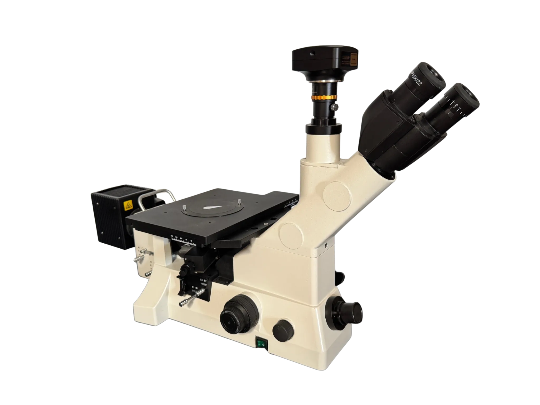
IM-5000, Mid-Range
Brightfield, darkfield, polarized light, and differential interference contrast (DIC) with infinite plan achromatic objectives. The contrast modes pull out relief, scratches, and fine second-phase detail that brightfield alone misses.
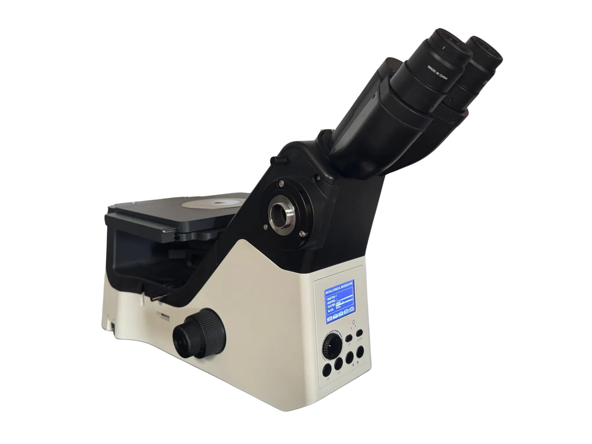
IM-7000, Premium
LM Plan S-APO objectives, advanced illumination, full BF/DF/POL/DIC suite. The right tool for research labs and any application where image quality is the limiting factor.
Optics Fundamentals
Two numbers determine what an optical microscope can actually show you: the objective's numerical aperture (N.A.) and the wavelength of light used to illuminate the sample. Magnification is a separate dial, and chasing magnification past what N.A. supports gives you a bigger picture of the same blurry information.
Numerical aperture and resolution
The numerical aperture measures the light-gathering capacity of the objective lens:
N.A. = μ · sin θ
where μ is the refractive index of the medium in front of the objective (μ = 1 for air, ~1.5 for immersion oil) and θ is the half-angle subtended by the objective at the specimen surface.
Resolution, the smallest distance at which two features can be seen as separate objects, follows from N.A. and the illumination wavelength:
Limit of Resolution = λ / (2 · N.A.)
Visible green light: λ ≈ 0.54 μm. With a high-N.A. air objective (N.A. ≈ 0.95), the limit is around 0.28 μm. With a high-N.A. oil immersion objective (N.A. ≈ 1.4), the limit drops to about 0.2 μm, the physical floor for visible-light microscopy.
An electron beam (λ ≈ 0.1 Å in an SEM) sidesteps the diffraction limit entirely, which is why SEM resolves down to angstroms.
Empty magnification
Total magnification is straightforward:
Total magnification = objective × eyepiece × tube factor
But beyond a certain point, adding magnification stops adding information. That ceiling is called empty magnification: the image gets bigger, but no new detail appears because the objective's N.A. has already exhausted its resolving power. A practical rule of thumb is that useful magnification tops out at roughly 1000× the objective's N.A.; pushing past that just produces softer, larger pixels. Pick the objective whose N.A. supports the magnification you actually need.
Optical filters
Filters in the light path sharpen the image for digital capture and reduce eye strain.
- Neutral density: reduce illumination intensity without changing color temperature
- Green monochromatic: a single wavelength produces sharper focus, especially helpful for monochrome image analysis
- Blue color correction: match a tungsten light source to daylight-balanced sensors (and vice versa)
- Color compensating: fine-tune residual color cast between illumination and sensor
Illumination Techniques
A metallurgical microscope uses reflected light: illumination travels down through the objective, reflects off the specimen, and returns through the objective to the eyepiece or camera. The illumination mode determines which features stand out. Switching modes is often the fastest way to reveal a feature that brightfield is hiding.
Brightfield (BF)
The default mode and the one most micrographs are shot in. Light enters at a high angle through the objective, reflects off flat surfaces, and returns to form a bright background. Features that scatter or absorb light (pores, edges, etched grain boundaries, second-phase particles) appear darker than the matrix. Brightfield is the right starting point for almost any sample.
Darkfield (DF)
A less common but powerful mode. Light bypasses the central optical path and travels down the outer rim of the objective, striking the sample at a low angle. Flat surfaces reflect that light away from the objective and stay dark; non-flat features (pores, edges, scratches, inclusions) scatter light back into the objective and appear bright on a black background. Darkfield can reveal microporosity, fine cracks, and surface scratches that brightfield washes out, and it makes preparation artifacts impossible to miss.
Polarized light
A polarizer and analyzer in crossed (90°) positions reveal optical anisotropy in the sample. Non-cubic crystals (titanium, zirconium, beryllium, magnesium, many ceramics) rotate the polarization plane and light up; cubic and amorphous materials extinguish to dark. Polarized light is the standard way to image grain structure in alpha-titanium, alpha-zirconium, and similar HCP metals that often will not etch cleanly with chemical reagents.
Differential Interference Contrast (DIC)
DIC uses a Nomarski prism between crossed polarizers to split the illumination into two beams that recombine at the focal plane. Height differences between phases appear as color or shading differences, giving the image a pseudo-3D look. DIC excels at revealing relief (height differences between phases), fine surface detail, and subtle features that brightfield contrast misses. It is the go-to mode for slightly relieved polished surfaces, weld fusion lines, and fine second-phase precipitates.
Switching modes is free information. When a feature looks ambiguous in brightfield, flip to darkfield or DIC before reaching for a different etchant or a higher-mag objective. The right illumination often turns a borderline image into a publication-ready one.
Quantitative Image Analysis
Words like "fine pearlite" or "moderate porosity" mean different things to different operators. Quantitative image analysis turns a micrograph into numbers that any reader can audit. It is essential for process development, quality control, failure analysis, and acceptance testing.
Stereology in one paragraph
A polished cross-section is two-dimensional, but most of the features you care about (grains, inclusions, pores, second-phase particles) are three-dimensional. Stereology is the mathematics that extracts 3D quantities (volume fraction, surface area per volume, particle count per volume) from 2D measurements (area fraction, intercept count, point count). The single most useful stereological identity:
VV = AA = PP
Volume fraction equals area fraction equals point-count fraction, provided enough fields are measured. This is why a manual point count on a 2D image yields the true 3D volume fraction of a phase.
Common measurements
- Point counting (PP): a regular grid is overlaid on the image; points falling inside the phase of interest are counted. Yields volume fraction.
- Linear intercept (NL): straight or circular test lines are placed on the image; the number of grain boundary intersections per unit length gives grain size.
- Area fraction (AA): the detected area of a phase divided by the field area. Yields volume fraction.
- Particle count (NA): number of features per unit area. Used for inclusion ratings and porosity.
- Mean free path (λ): average edge-to-edge spacing between particles, perpendicular to the working direction. λ = (1 − AA) / NL.
- 95% confidence interval: t · s / √n, where s is the standard deviation across n fields. Always report it; a phase fraction without a CI is not a measurement.
Manual or automated
Both are valid. Manual point counting against a reticle (ASTM E562) is auditable and works on any microscope. Automated image analysis (ASTM E1245, E1382) is faster, scales, and removes operator-to-operator variability, but it depends entirely on the polished and etched surface, because the software is detecting contrast, not actual features. Bad preparation produces bad analysis whether the operator or the computer is counting.
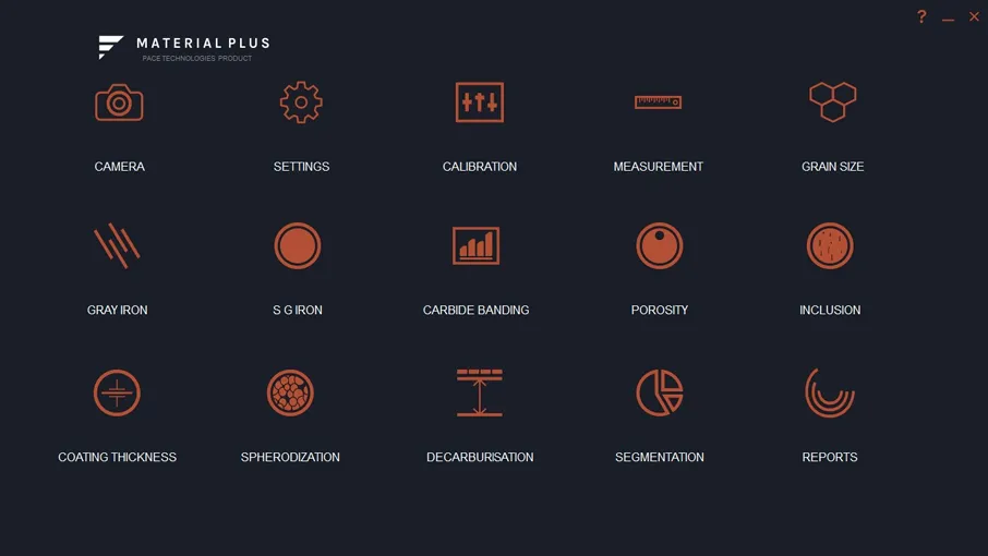
PACE Material Plus image analysis software, with optional WELD CHECK and Hardness PRO modules.
PACE supplies Material Plus for ASTM-compliant automated analysis (grain size, phase, porosity, inclusion rating, decarburization, coating thickness), along with the WELD CHECK and Hardness PRO add-on modules.
Standard ASTM Procedures
Each measurement below is covered by a published ASTM (or equivalent) standard. The standard defines the method, the field count, the magnification, and the reporting conventions; write the standard number on the report, not just the result.
| Measurement | Standard(s) | What it measures |
|---|---|---|
| Grain size | ASTM E112, E930, E1181, E1382 | Average grain size; ALA (as-large-as) grain size; duplex grain sizes; automated grain size |
| Phase / second-phase content | ASTM E562, E1245 | Volume fraction by point count (manual) or automated image analysis |
| Nodularity (cast iron) | ASTM A247 | Graphite form, distribution, and size in iron castings |
| Porosity | ASTM E562, E1245 | Volume fraction of voids |
| Inclusion rating | ASTM E45, E1245 | Type, size, and severity of non-metallic inclusions in wrought steel |
| Decarburization | ASTM E1077 | Depth of carbon loss at the surface of steel |
| Coating thickness | ASTM B487 | Metal and oxide coating thickness by cross-section microscopy |
| Weld analysis | SAE, AWS standards (e.g., AWS B4.0) | Throat, leg, root penetration, HAZ depth and area |
Grain size (ASTM E112, E930, E1181)
A grain is one crystal in a polycrystalline material. Grain size is intrinsically three-dimensional but measured on a 2D section. ASTM E112 specifies three procedures:
- Comparison: overlay the micrograph against ASTM chart plates at matching magnification. Fast, well-suited to fully recrystallized equiaxed grain structures.
- Planimetric (Jeffries): a known area (typically 5000 mm² of the printed image) is laid over the micrograph; full grains plus half of the intercepted grains times the Jeffries multiplier gives the grain count. Requires at least 50 grains per field.
- Intercept (Heyn): straight or circular test lines are drawn across the image; counted grain boundary intersections give grain size. The recommended method for non-equiaxed structures.
Always exclude twin boundaries from the count; they are coherent boundaries within a single grain, not grain boundaries. ASTM E930 handles very coarse structures where E112 has too few grains per field; E1181 handles duplex (bimodal) grain populations; E1382 covers automated image analysis.
Phase analysis (ASTM E562, E1245)
A phase is a physically homogenous, distinct constituent. The two governing standards are E562 (manual point count) and E1245 (automatic image analysis for inclusions and second-phase constituents). Either yields volume fraction with a stated confidence interval. Use E562 when audit traceability matters most; use E1245 when speed and sample count matter most. Both depend on a clean polish and a sharply contrasting etch.
Nodularity (ASTM A247)
ASTM A247 classifies graphite in cast iron along three axes: form (Types I–VII, with I–VI for nodular/spheroidal graphite and VII for gray-iron flake), distribution (letters A–E), and size (numbers 1–8, largest to smallest). Compare against ASTM Plates I, II, and III at the standard magnification. Software-based nodularity classification (Material Plus and similar) accelerates the count and removes operator drift.
Porosity (ASTM E562)
Porosity is measured as a volume fraction. Manual point count (E562) overlays a grid (16, 25, 49, or 100 points are the standard arrays) on each of n fields, counts the points falling inside pores, and computes VV = PP ± 95% CI. Automated image analysis (E1245) does the same operation on detected pixels. For sintered powder metallurgy parts, thermal spray coatings, and castings, porosity is one of the most consequential numbers you can report.
Inclusion rating (ASTM E45)
ASTM E45 characterizes non-metallic inclusions in wrought steel using the JK rating system:
- Type A, Sulfide: stringers, light gray under brightfield
- Type B, Alumina: aligned clusters of at least three round/angular oxide particles (aspect ratio < 2) parallel to the working direction
- Type C, Silicate: stringers, black under brightfield (the easy way to tell A from C)
- Type D, Globular oxide: isolated round oxides, not aligned
Each type is then rated by thickness (T = thin, H = heavy) and severity level based on count or length in a 0.50 mm² field. The result is a compact code (e.g., "A2T, B1H, C1T, D1T") that quality assurance tracks across heats and lots.
Decarburization (ASTM E1077)
Decarburization is the loss of carbon at a steel surface, usually from heat-treat atmosphere or hot-working. It changes hardness, fatigue life, and wear behavior at the part's surface. ASTM E1077 defines:
- Complete decarburization: surface ferrite only, no pearlite
- Partial decarburization: reduced carbon, mixed ferrite + pearlite zone
- Total depth: perpendicular distance from the surface to where bulk carbon content is restored
- Average depth: mean of at least 5 measurements
- Maximum depth: the largest single measurement
All four are read directly from a properly etched cross-section. For heat-treated steels, the presence of non-martensitic structure in the partial zone is used to identify the boundary.
Coating thickness (ASTM B487)
ASTM B487 specifies the cross-sectional microscopy method for measuring metal and oxide coatings. The non-negotiable requirements: the cross-section must be perpendicular to the coating (any tilt inflates the apparent thickness), the surface must be flat across the entire field so the boundaries are sharply defined, and the section must be free of deformation, smearing, or rounded edges. Mount the part so the coating is in compression during sectioning and grinding, and use edge-retention compounds and resin systems suited to the substrate. Coating measurements live or die on edge quality.
Weld analysis
No single ASTM standard covers all weld measurements; SAE and AWS publish the applicable specs. Common measurements include throat dimension (foot of fillet to face), leg length (root of joint to surface intersection), root penetration, joint penetration angles, HAZ depth and area, and phase counts inside the fusion zone and HAZ. PACE supplies the WELD CHECK module for Material Plus to automate the standard weld geometry measurements.
Universal Best Practices
These habits apply to any microscopy or image-analysis session.
Before the session
- Confirm preparation quality at low magnification first; a remaining scratch at 50× will only get worse at 500×
- Calibrate the stage micrometer at every objective you plan to use; recalibrate after changing eyepieces, cameras, or zoom settings
- For image analysis, verify that the calibration file matches the objective in use; wrong calibration is the most common silent error
- Clean objectives gently with lens tissue and approved cleaner; never with paper towel or shop rag
During the session
- Start at the lowest useful magnification and step up only as needed. Empty magnification wastes time without adding information.
- When a feature looks ambiguous, change illumination mode before changing objectives or etchants
- Use Köhler illumination for the cleanest image (field and aperture diaphragms set per the microscope manual)
- For quantitative work, take enough fields to drive the 95% CI below your acceptance threshold (typically 5 to 12 fields, more for low-area-fraction phases)
After the session
- Save raw images alongside any analysis output; the standard ASTM reports a number, but the image is the evidence
- Record the magnification, illumination mode, etchant, and calibration file in the image metadata or filename
- Cover the microscope and store immersion-oil objectives wiped clean to prevent oil migration into the lens cement
The micrograph is the audit trail. A quantitative result without an attached image cannot be re-checked, re-analyzed, or compared against future heats. Save the image, write the standard on the report, and the result will stand up to any review.
Troubleshooting
Most microscopy problems trace back to preparation, calibration, or illumination, in that order. Use the table below before assuming the microscope or the software is at fault.
| Problem | Common causes | Solutions |
|---|---|---|
| Image looks soft or out of focus at high magnification |
|
|
| Features in brightfield look ambiguous or low-contrast |
|
|
| Grain size or phase count drifts between operators |
|
|
| Image analysis software detects scratches as inclusions |
|
|
| Coating thickness measurement varies along the length |
|
|
| Polarized light gives no contrast on a known anisotropic alloy |
|
|
Frequently Asked Questions
What is "empty magnification" and how do I avoid it?
Empty magnification is the point where increasing magnification no longer adds detail because the objective's numerical aperture has already exhausted its resolving power. As a working rule, useful magnification tops out at about 1000× the objective's N.A.; so a 0.65-N.A. objective is usefully scaled to around 650×, and pushing higher just produces softer, larger pixels. The fix is to step up to a higher-N.A. objective (or oil immersion at the top end), not to add eyepiece or camera magnification.
When should I use darkfield instead of brightfield?
Use darkfield when you need to highlight non-flat features (porosity, fine cracks, scratches, inclusions, surface debris) that wash out in brightfield. The dark background makes small light-scattering features unmistakable. Darkfield is also the fastest way to expose remaining preparation artifacts; if a polish looks clean in brightfield but lights up in darkfield, the polish is not finished.
My titanium / zirconium sample will not etch. Am I doing something wrong?
Often nothing. Titanium, zirconium, beryllium, and many other HCP metals are chemically resistant and resist conventional chemical etching. Use polarized light on the as-polished (or vibratory-polished) surface: anisotropic grains light up in shades determined by their orientation, with no etchant required. A small amount of Kroll's reagent can help on Ti alloys, but POL is often the cleaner answer.
How do I measure grain size? (ASTM E112)
ASTM E112 specifies several procedures; the two most common are the planimetric (Jeffries) method and the linear intercept (Heyn) method. Planimetric: count grains entirely inside a known test area plus half-grains crossing the boundary, divide by area, multiply by the magnification factor to get grains per mm², then look up the ASTM grain size number from the standard's table. Linear intercept: count grain-boundary intersections along a test line of known length, divide by line length × magnification, get intercepts per mm, look up the ASTM number. Both methods require a properly etched specimen with clear, unambiguous grain boundaries. Statistical defensibility requires multiple fields; report grain size to one decimal place plus the 95% confidence interval. PACE Material Plus runs both methods automatically and applies the magnification correction for you.
How do I count inclusions or porosity? (ASTM E45)
ASTM E45 covers inclusion rating for steels and similar alloys. The standard requires 100× magnification (some methods use 500×), a specimen polished to a true 1 μm or finer finish without etching, and either chart-comparison rating (Method A, the traditional method) or automated image analysis (Method D, increasingly preferred). The four inclusion types are A (sulfides), B (alumina stringers), C (silicates), and D (globular oxides), each rated for thin (1) or heavy (2) on a 0–5 severity scale per stringer per 0.5 mm². The polish step is the critical control: pulled inclusions read as missing material, smeared inclusions read as bigger than they are, and embedded abrasive reads as inclusions that are not actually there. Best practice for E45 work: vibratory polish before measurement to eliminate residual deformation.
How many fields do I need to measure for a defensible phase count?
It depends on the phase fraction. ASTM E562 recommends starting with 5 fields and adding more until the 95% confidence interval drops below your acceptance threshold (often expressed as relative accuracy, %RA, of 10% or better). For phases above ~10% area fraction, 5 to 12 fields is usually enough. For low-fraction phases (inclusions, trace porosity), 20 or more fields may be required to drive the CI down. The standard requires that you report the CI alongside the result; a phase fraction without a CI is not a measurement.
Manual point count or automated image analysis, which should I use?
Both are valid, and both depend on a clean polish and etch. Manual point count (ASTM E562) is the audit-friendly default and works on any microscope. Automated image analysis (ASTM E1245/E1382, run with PACE Material Plus or equivalent) is much faster, scales to hundreds of fields, and removes operator-to-operator variability, but it detects pixel contrast, not features, so any preparation artifact that contrasts with the matrix gets counted. For high-volume QC, automation pays for itself in weeks; for one-off failure analysis, manual point counting is often quicker to set up correctly.
Why do my coating thickness measurements vary so much?
Almost always one of three causes: the cross-section is not perpendicular to the coating (any tilt inflates the apparent thickness), the edge is rounded from poor edge retention during grinding, or the coating was smeared by sectioning or grinding damage. The fix is process: mount so the coating is in compression during the cut, use an edge-retention mounting compound, and finish to a fine final abrasive before measuring. ASTM B487 requires a sharply-defined boundary; if the boundary is fuzzy, the number cannot be trusted.
How do I store a polished or etched sample between prep and imaging?
For short-term storage (minutes to hours): rinse with ethanol, dry with compressed air, and place in a covered petri dish or specimen box with a desiccant pack. For overnight to several days: apply a clear protective lacquer to the polished face after final cleaning; the lacquer comes off with acetone before imaging. For long-term archival: photograph the microstructure first because it will change, then mount the specimen face-down in a clean dish with desiccant and store away from light and humidity. Carbon steels and copper alloys oxidize most aggressively; stainless steels and titanium alloys hold their polish longest. Never store an etched sample unprotected; the etched surface is chemically reactive and will continue to darken even in clean air.
What's Next: Material-Specific Interpretation
The standards in this guide tell you how to measure a microstructure. The material-specific guides tell you what the result means: which phases to expect, what cooling rate they imply, which etchant brings them out, and which defects matter for that alloy class. Start with the alloy you are actually working on.